
Data Modeling for Analytics Engineers: The Complete Primer
The best data models make it hard to ask bad questions and easy to answer good ones.


Your data model isn't about tech specs. It's about thinking like a business. Consider it the blueprint for your entire analytics house. If the blueprint's chaotic, your house crumbles. If it's structured and organized, your team finds insights fast.
You’re staring at a spreadsheet full of customer orders, product prices, and sales dates. It’s messy. Your “dashboard” is slow. You’ve tried to answer a simple question like: How much revenue did pizza make last quarter? and ended up with numbers that don’t add up. Why? Because your data model is a pure mess.
In this blog post - adapted from a chapter of my book Analytics Engineering with Microsoft Fabric and Power BI, which I’m writing with Shabnam Watson for O’Reilly, I’ll walk you through the core data modeling concepts that every analytics engineer should know. Forget Power BI and Microsoft Fabric for a second. This is about core principles - the why behind models. These ideas work regardless of the tool.
Let’s start by introducing the challenge. Imagine you run a tiny pizzeria. Your “database” is a single Excel sheet: Order ID, Customer Name, Address, Pizza Type, Quantity, Price. Looks simple enough, right? The problem? John Smith’s address is repeated in every single order. If he moves, you’ve got to edit 37,000 rows of orders just to update his address. Doesn’t look smart, right?
Your data model is the fix. It literally says: Customers live in their own table. Orders link to Customers without copying addresses. It’s not about how you’re going to visualize the data. It’s about organizing it so the data makes sense when you ask questions.
However, data modeling begins long before your data is stored in a spreadsheet or in a real database. In the following sections, we will introduce core data modeling concepts - the ones that should be implemented in every single data modeling scenario, regardless of the modeling approach you plan to take or the tool you are going to use for the physical implementation.
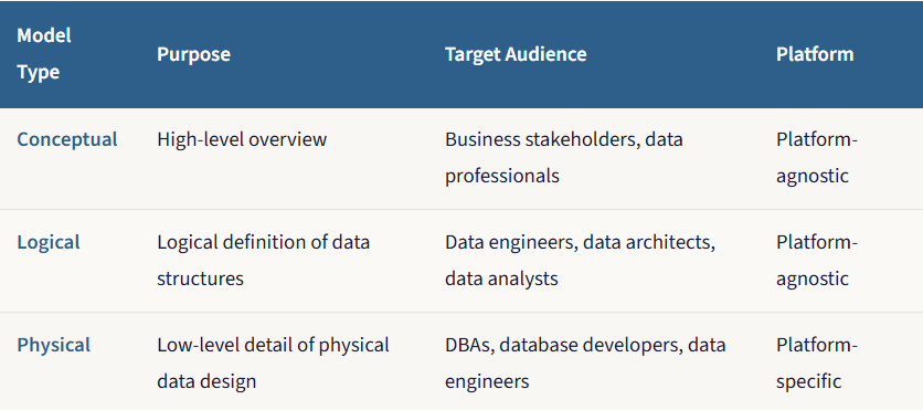
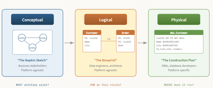
Just as an architect doesn’t go straight from an idea to a finished building, a data modeler doesn’t create a database schema in a single step. The process progresses through three levels of increasing detail, each serving a distinct purpose and audience. Think of it as progressing from a conceptual sketch, to a detailed architectural blueprint, to a final construction plan used by the builders.
Conceptual model: The napkin sketch
Every great data model begins not with code or tables, but with a conversation. The conceptual model is the very first, highest-level view of your data. It’s completely non-technical and focuses solely on understanding and defining the business concepts and the rules that govern them.
The conceptual model identifies the main things or entities a business cares about and how they relate to each other. It creates a vocabulary for talking with business stakeholders to ensure you’re speaking the same language.
Imagine an architect meeting with a client at a coffee shop. The client might say something like: I want a family home that feels open and connected. The architect takes a napkin and draws a few bubbles: Kitchen, Living Room, Bedrooms, and draws lines between them labeled “connects to” or “is separate from.” There are no dimensions, no materials, no technical details. It’s just about capturing the core idea and ensuring that everyone agrees on the fundamental concepts. That napkin sketch is the conceptual data model.
Let’s look at a real example - events at a stadium. In a conceptual model for this scenario, you’d identify several entities: Stadium, Event, Customer, Attendee, and Ticket. You’d also notice how these entities are interconnected. This high-level overview provides a simplified picture of the business workflow within the organization.
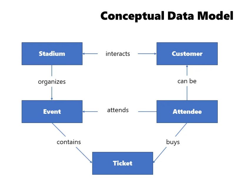
A Stadium has a name and is located in a specific country and city, which uniquely identifies it. This Stadium may host many events, and there can be many attendees coming to these events. An Event cannot exist outside of the Stadium where it is scheduled. An event can be attended by an attendee, and there can be many attendees for one event. An Attendee is the entity that attends the event. They can also be a Customer of the Stadium entity - for example, by visiting a stadium museum or buying at a fan shop - but that doesn’t make them an attendee of a specific event. Finally, a Ticket represents confirmation that the attendee will attend a specific event. Each Ticket has a unique identifier, and one Attendee can purchase multiple Tickets.
Now, you might be wondering: why is this important? Why should someone spend time and effort describing all the entities and relations between them?
Remember, the conceptual data model is all about building trust between business and data personas - ensuring that business stakeholders will get what they need, explained in a common language, so that they can easily understand the entire workflow. Setting up a conceptual data model also provides business stakeholders with a way to identify a whole range of business questions that need to be answered before building anything physical. Questions like: Are the Customer and Attendee the same entity (and why are they not)? Can one Attendee buy multiple Tickets? What uniquely identifies a specific Event?
Additionally, the conceptual data model depicts very complex business processes in an easier-to-consume way. Instead of going through pages and pages of written documentation, you can take a look at the illustration of entities and relationships, all explained in a user-friendly way, and quickly understand the core elements of the business process.
Logical model: The blueprint
Once business and data teams align on the conceptual data model, the next step is designing a logical data model. In this stage, we are building upon the previous step by identifying the exact structure of the entities and providing more details about the relationships between them. You should identify all the attributes of interest for each entity, as well as relationship cardinality.
Note that, just as during the conceptual data modeling phase, we’re still not talking about any specific platform or solution. The focus is still on understanding business requirements and how these requirements can be efficiently translated into a data model.
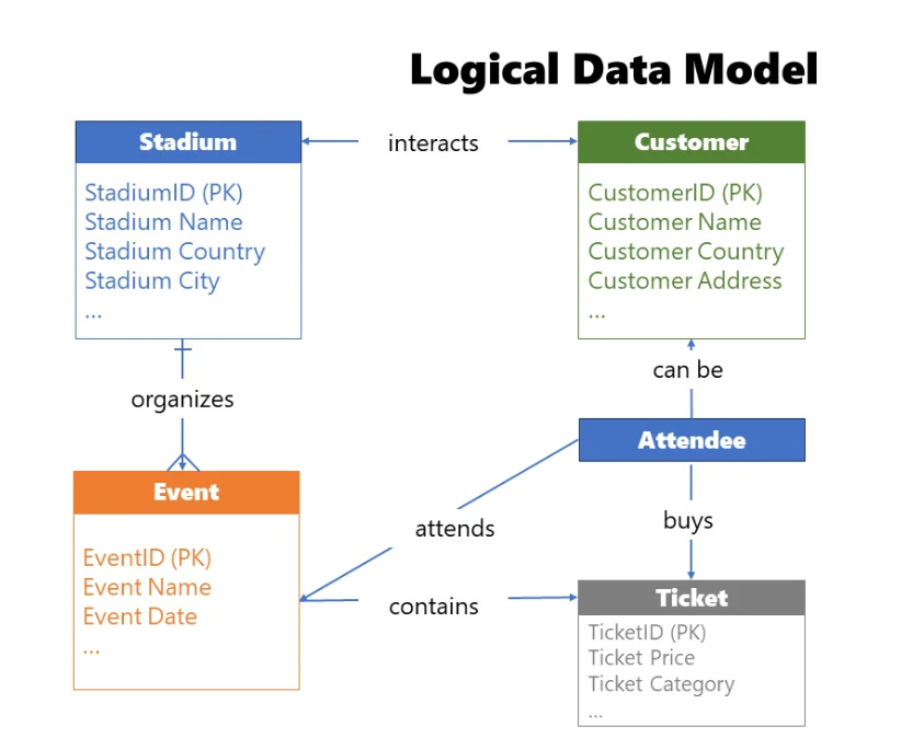
There are several steps to ensure that the conceptual model successfully evolves into a logical model. You need to identify entity attributes - the specific data points each entity should contain. Then identify candidate keys - which attribute, or set of attributes, uniquely identifies a specific entity. From there, choose primary keys based on the findings from the previous step. You’ll also apply normalization or denormalization as appropriate (more on that later). Next, set relationships between entities, validating how entities interconnect and, if needed, breaking down complex entities into multiple simpler ones. Then identify the relationship cardinality — defining how many instances of one entity relate to instances of another. There are three main types: one-to-one (1:1), one-to-many (1:M), and many-to-many (M:M). Finally, and critically, iterate and fine-tune. In real life, it’s almost impossible to find a data model that suits everyone’s needs immediately. Ask for feedback from business stakeholders and fine-tune the logical data model before materializing it in physical form.
The potential gains of the logical model are significant. First, it serves as the best quality assurance test, identifying gaps and issues in understanding the business workflow, thereby saving you a significant amount of time and effort in the long run. It’s much easier and less costly to fix issues at this stage, before locking into a specific platform. Building a logical data model can be considered part of the agile data modeling cycle, which ensures more robust, scalable, and future-proof models. And ultimately, it serves as a blueprint for the final physical implementation.
Physical model: The construction plan
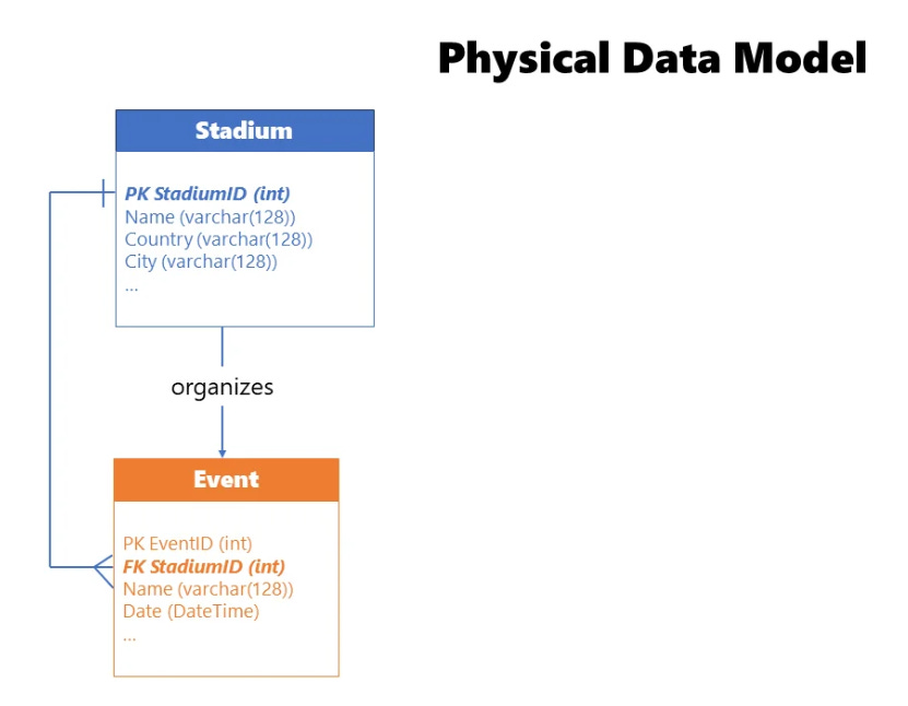
A physical data model represents the final touch: how the data model will actually be implemented in a specific database. Unlike conceptual and logical data models, which are platform and solution-agnostic, physical implementation requires defining low-level details that may be specific to a certain database provider.
There’s a whole list of necessary steps to make your physical data model implementation successful. You need to choose the platform - this decision shapes your future design principles. Then translate logical entities into physical tables - since a real database doesn’t support the abstract level of a logical entity, you need to define the data type of each attribute: whole number, decimal number, or plain text. Additionally, each physical table should rely on keys (primary, foreign, unique) to ensure data integrity.
You must also establish relationships based on the key columns. Apply normalization or denormalization as appropriate - remember, in OLTP systems, tables should be normalized (typically to 3NF) to reduce redundancy and support write operations efficiently, while in OLAP systems, data may be denormalized to eliminate joins and make read operations more performant.
Define table constraints to ensure data integrity - not just keys, but logical checks too. For example, if your table stores student grades in the range of 5 to 10, why not define that constraint on the column, preventing the insertion of nonsensical values?
Create indexes and/or partitions - these are special physical data structures that increase the efficiency of the data model. Table partitioning, for example, splits one big table into multiple smaller sub-tables, reducing scanning time during query execution. A classic approach is partitioning by calendar year. And finally, extend with programmatic objects - stored procedures, functions, triggers — that are de facto standard in almost every data platform solution.
The main benefit of the physical data model is to ensure efficiency, optimal performance, and scalability. When we talk about efficiency, we have in mind the two most precious business assets: time and money. Unless you think that time = money, then you have only one asset to consider. The more efficient your data model, the more users it can serve, the faster it can serve them, and that, in the end, brings more money to the business.
Why bother with all three? Because fixing a gap in the conceptual model costs a conversation. Fixing it in the physical model costs a sprint. The earlier you catch issues, the cheaper they are to resolve.
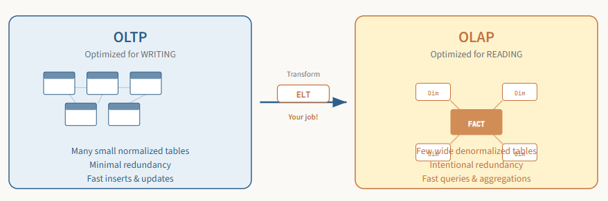
OLTP vs. OLAP: Writing vs. Reading
Online Transaction Processing Systems (OLTP)
To be a successful analytics engineer, you must first understand where your data comes from. The vast majority of business data isn’t created for analytics. It’s created by applications that run the daily operations of the business: a point-of-sale system, a customer relationship management (CRM) tool, an e-commerce website’s backend database, and many more.
These source systems are called online transaction processing (OLTP) systems. They are designed and optimized for one primary goal: to process a high volume of transactions quickly and reliably. OLTP systems need to instantly confirm a customer’s order or update their shipping address. Speed and data integrity for writing data are paramount.
To achieve this, OLTP systems use a relational data model that is highly normalized. Let’s dive deep into what that actually means.
Normalization: The library card catalog
Normalization is the process of organizing data in a database to minimize data redundancy and improve data integrity. In simple terms, it means you don’t repeat information if you don’t have to.
Imagine a library in the pre-computer era. Each and every book has an index card. If the author’s full name, nationality, and date of birth had to be written on every card for every book an author wrote, it would be tedious. You’d be writing “William Shakespeare, English, 1564-1616” on the cards for Hamlet, Macbeth, and Romeo and Juliet. And if you discovered a mistake in Shakespeare’s birth year, you’d have to find and correct every single card for every book he wrote. It’s almost guaranteed you’d miss one.
A smart librarian would use normalization. They would create a separate Authors card catalog. The card for Hamlet would just say “Author ID: 302.” You would then go to the Authors catalog, look up ID 302, and find all of William Shakespeare’s details in one single place. If you need to make a correction, you only have to do it once.
Normal Forms
This is the essence of normalization: breaking data down into many small, discrete tables to avoid repeating ourselves. The rules for doing this are called normal forms (1NF, 2NF, 3NF...). There are seven normal forms in total, although in most real-life scenarios, normalizing data to the third normal form (3NF) is considered optimal.
Let’s briefly break down the key principles behind the first three normal forms. First normal form (1NF) eliminates repeating groups. Each cell should hold a single value, and each record should be unique. Second normal form (2NF) builds on 1NF and ensures that all attributes depend on the entire primary key - this is mainly relevant for tables with composite keys. Third normal form (3NF) builds on 2NF and ensures that no attribute depends on another non-key attribute. This is the library example: AuthorNationality doesn’t depend on the book; it depends on the author. So, you move AuthorNationality to the Authors table.
Let’s look at a before-and-after example. Imagine a non-normalized spreadsheet for tracking orders: OrderID, OrderDate, CustomerID, CustomerName, CustomerCity, ProductID, ProductName, Qty, UnitPrice - all in one flat table. Notice all the repetition? John Smith’s name and city are repeated. Widget A’s name and price are repeated. To update Widget A’s price, you have to change it in two places, and that’s just in a tiny sample.
To normalize this data to 3NF, we break it down into four separate tables: a Customer table (CustomerID, CustomerName, CustomerCity), a Product table (ProductID, ProductName, UnitPrice), an Orders table (OrderID, OrderDate, CustomerID), and an OrderDetails table (OrderID, ProductID, Qty). Now if John Smith moves to Los Angeles, we update his city in exactly one place. If the price of Widget A changes, we update it in exactly one place. This is perfect for the OLTP system.
However, life is not a fairy tale. And here’s the twist. While this normalized structure is brilliant for writing data, it’s inefficient for analyzing it. To answer a simple question like “What is the total sales amount for products in the ‘Widgets’ category to customers in New York?” you’d have to perform multiple complex JOIN operations across all these little tables. With dozens or even hundreds of tables, these queries become incredibly slow and a nightmare for your business users to write.
This leads us to the core job of an analytics engineer: transforming data from a model optimized for writing (OLTP) to one optimized for reading (OLAP).
Online Analytical Processing Systems (OLAP)
If OLTP systems are for running the business, online analytical processing (OLAP) systems are for understanding the business. Our main goal as analytics engineers is to build OLAP systems. These systems are designed to answer complex business questions over large volumes of data as quickly as possible.
Denormalization: The strategic reversal
Let’s kick it off by explaining denormalization. As you may rightly assume, with denormalization we are strategically reversing the process of normalization that we previously examined. We intentionally re-combine many small tables into a few larger, wider tables, even if it means repeating some data and creating redundancy.
Denormalization is essentially a trade-off: we are sacrificing a bit of storage space and update operation efficiency to obtain potentially massive gains in query performance and ease of use. Denormalization is one of the core concepts for implementing dimensional data modeling techniques, covered next.
Dimensional modeling: The Star schema and beyond
A dimensional model represents the gold-standard paradigm when designing OLAP systems. Before we explain the dimensional aspect, let's have a brief history lesson. Ralph Kimball's book The Data Warehouse Toolkit (Wiley, 1996) is still considered a dimensional modeling bible. In it, Kimball introduced a completely new approach to modeling data for analytical workloads - the so-called bottom-up approach. The focus is on identifying key business processes within the organization and modeling these first, before introducing additional business processes.
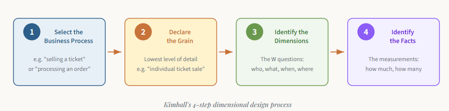
Kimball’s approach is elegant in its simplicity. It consists of four steps, each based on a decision:
