


If you worked with Microsoft Power BI before Microsoft Fabric was announced, you might be (rightly) wondering – what’s all the fuss about? Nothing has really changed from the UI perspective, and all of the features and functionalities are still available as they were in the pre-Fabric era (by the way, you’ll see me using this phrase multiple times throughout this article).
And, you are absolutely right! Fabric user interface was built on top of the existing Power BI Service UI. To be more precise, all the other experiences and workloads, such as Data Engineering, Data Warehouse, or Real-time Intelligence, were incorporated into the well-known Power BI experience. Hence, once you navigate to the Fabric home page and choose Power BI from the home page, things will look quite familiar to anyone who has ever logged in to Microsoft Power BI Service.
Does this mean that Power BI remained the only unchanged island in the vast sea of innovations that Microsoft Fabric introduced? Absolutely not!
In this article, I will discuss how pre-Fabric Power BI workloads were integrated into the new ecosystem, as well as introduce brand-new concepts and features that Microsoft Fabric brought into the Power BI game. I’ll also bring some points to consider when planning your future analytics solutions and examine various scenarios for leveraging Power BI capabilities in the era of Microsoft Fabric.
This is the excerpt from the early release of the “Fundamentals of Microsoft Fabric” book, that I’m writing together with Ben Weissman for O’Reilly. You can read the early release, which is updated chapter by chapter, here.

Power BI Workloads in the Pre-Fabric Era
Dear reader, if you have never used Microsoft Power BI, I suggest you take one step back and find the Power BI learning resource that best suits your needs - be it a book, an online course, or live training.
In this section, I’m taking you on a 10.000-feet tour of Power BI and its main components so you can continue your Fabric journey well-equipped and feel more comfortable diving deeper into specific concepts and features of Power BI if necessary. I will also share some additional resources that we might consider useful for learning Power BI.
In a nutshell, Power BI represents a suite of tools and services for business reporting. The main mantra of Power BI is: “5 minutes to WOW!” To put it simply - there should be no longer than 5 minutes from the moment you connect to any of the various disparate data sources until you have nice-looking and visually appealing charts that provide insight from the underlying data. Of course, in reality, it’s usually more than 5 minutes, but the emphasis here is on the ease of use and pace of the development process.
I am not exaggerating if I say that Power BI has managed to live up to its promise. In the end, Gartner recognized Microsoft Power BI as an undisputed leader in Analytics and Business Intelligence Platforms “magic quadrant” for multiple years in a row. More details can be found here.
In the context of Fabric, we are talking about Microsoft Power BI as a mature and well-established product that democratized data analytics workloads. The level of Power BI adoption is already high, while the vibrant community of data professionals using Power BI ensures that the product gets more and more popular over time.
To understand what has changed in Power BI workloads from a Fabric perspective, we first need to examine typical workflows in the pre-Fabric era.
Let’s kick it off with storage modes – in simple words – a storage mode determines how your data is stored in Power BI semantic models. There are three main options to choose from: Import, DirectQuery, and Dual. I’ll first introduce the Import mode, as a default storage mode in Power BI.
Import mode for blazing-fast performance
When using Import mode, once you connect to the data source(s), Power BI creates a local copy of the data and stores this local copy in the instance of a tabular Analysis Services model. For those of you who haven’t heard about the Analysis Services - don’t worry - this is an analytical data engine developed by Microsoft and used in numerous Microsoft’s business intelligence solutions since the beginning of this century.
You can apply various transformations, such as replacing values, removing duplicates, adding new columns, to shape your data and implement additional business logic to enrich the existing data model. The important thing to keep in mind is that, since you are working with the local copy of the data, all the transformations and changes you’ve applied are relevant only to this local copy in the Analysis Services tabular that Power BI uses for storing the data. Hence, you don’t need to worry that changes made to the Excel file stored in Power BI will be pushed back to the original Excel file stored on your local drive.
Once the data is stored in the Analysis Services Tabular, Power BI keeps it in the cache memory, in the columnar, in-memory database, called VertiPaq. As you may notice in the illustration below, all queries generated by the Power BI report will then retrieve the data from this in-memory storage, without even “knowing” about the “real” data source. In this scenario, the only data source is the instance of Analysis Services Tabular, and all the queries will refer to it for data retrieval.

Since the data is stored in cache memory, the main advantage of using Import mode is the best possible performance of DAX queries. On the flip side, there are certain downsides when going the Import mode route. The most obvious one is data duplication because we are essentially creating a copy of the data from the data source in Power BI’s Tabular database, as well as data latency, which means that when you import the data from the original data source into Power BI, this is nothing else but the data snapshot as of the moment you imported it into Power BI.
Let us illustrate this: imagine that you’ve imported data from the Excel file stored on your local PC, on Monday at 9 AM. At that point in time, you had 1000 records in this Excel file. What happens if you insert another 100 records in the Excel file after Monday 9 AM? Well, Power BI doesn’t have an idea about that until you refresh the local copy of the data stored in Power BI. This means, that between Monday 9 AM and the next data refresh (let’s say on Tuesday 9 AM), Power BI will query and display the data as of Monday 9 AM.
To wrap up – Import mode provides the best possible experience from the performance point of view, but it also comes with two considerable shortcomings: data duplication and data latency. In addition, depending on the capacity size, there is a hard limit on the maximum semantic model size - for example, if you’re using an F2, F4, or F8 capacity, the maximum model size is 3GB; it’s 5GB on F16, 10GB on F32, 25GB on F64, and so forth. This limit applies to an individual semantic model, not the sum of the memory footprint of all the models in the capacity.
DirectQuery mode for real-time reporting
DirectQuery mode solves these shortcomings of the Import mode.
As you can see in the illustration below, there is no duplication, as no data is moved from the original data source into Power BI. Power BI stores metadata only and retrieves the necessary data directly from the source at the query time. This means that data resides in its original data source before, during, and after the query execution.
There is no latency, either. Since Power BI retrieves the data at the query time, whatever data is available at the source at the query time, will also be available in the Power BI report.
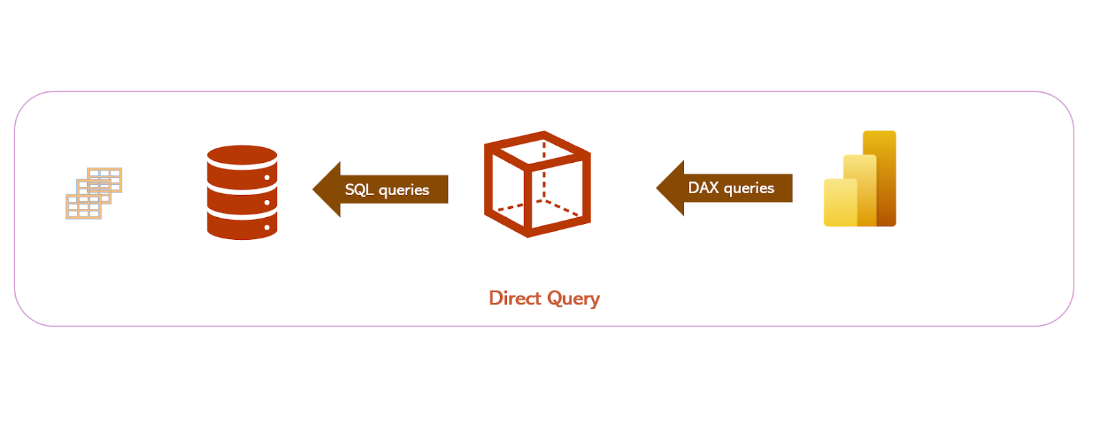
As you may notice in the same illustration, all DAX queries generated by Power BI are simply translated on the fly into the SQL code and executed directly on the source database.
This is great, isn’t it?! No data duplication and no data latency, so why don’t we simply switch all our semantic models to DirectQuery? The answer is fairly simple: in most cases, the performance of DirectQuery semantic models is significantly worse than in Import mode. First of all, it highly depends on the data source performance capabilities, as well as network bandwidth and latency. Throw in the potential bottleneck of On-premises data gateway and we are talking about the performance degradation in the order of magnitude, which usually goes beyond multiple times slower report over the same data compared to the Import mode.
Hence, choosing between Import and DirectQuery mode is usually a trade-off between the performance and real-time reporting requirements:
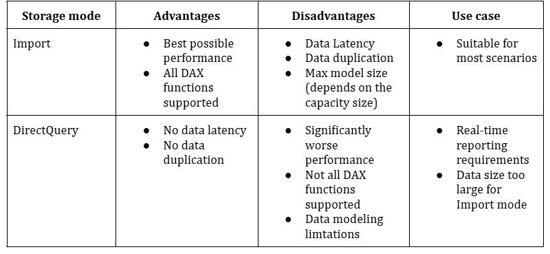
Additionally, not all DAX functions are supported in the DirectQuery mode. Certain DAX functions can’t be “translated” to SQL language, thus preventing the usage of the DirectQuery storage mode.